Hi! How you doing? Today we will be doing hyperparameter tuning with the help of the RandomisedSearchCV algorithm.

What are Hyperparameters actually?

Let’s see this way when using a machine learning algorithm, there are various parameters associated with the instance or the method we using of a particular algorithm By default, it is provided, which gives significantly good results. However, if we want to increase the accuracy of the results, we have to make some tweaks to the default parameters. And the process of tuning such parameters with the hope of better accuracy of the given model using a particular algorithm instance can be called Hyperparameter Tuning. If it looks like Jargon, we will look at an example of the default parameter of the Support Vector Machine Classifier SVC instance.

In the above example, when we see the parameters of the SVC instance, we get the default parameters as mentioned above. So when we instantiate the SVC instance, the default parameters are passed in it. But when we visit the official documentation of SVC, we see a bunch of these parameters can be passed as a dictionary or list. So, we use that feature of such flexibility of these parameters and try a different set of parameters and find the best parameters that give the best results.

So, what we do is take a dataset and work on it and find the accuracy by default parameters and then tune few parameters to increase the score.

For this task, we will be using Jupyter Notebook. If you like doing it in a local machine it's okay, but I highly suggest using the online Jupyter Notebook. Colab by Google is a very good resource that we can use for free and Deepnote is another alternative to Google Colab. Here, I personally will be using Deepnote.

    #importing required moduls.
    import pandas as pd #for tabular data frame analysis
    import numpy as np. #Form mathematical Manipulation
    import matplotlib.pyplot as plt #for data visulaization
    import seaborn as sns #Seaborn is developed on top of matplotlib library

So, we need a dataset for it. There are various datasets available in kaggle. And we take a simple dataset from Kaggle Heart Disease Dataset.

#loading dataset
df = pd.read_csv('./heart.csv') #The dataset is downloaded and saved to root folder.
df.head()

After this, we get the first five rows of the dataset.

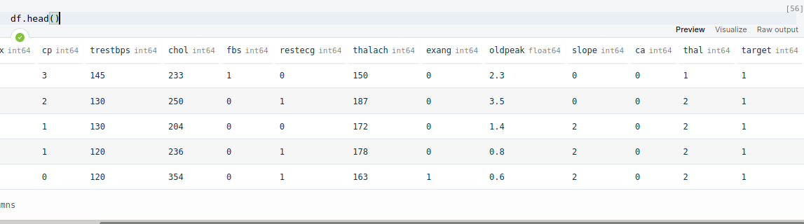However, if we look closely to Target feature, we see all 1's and if we make even close oversvation with df['target'], we see a pattern that first half of the dataset has 1 value in target feature and remaining has 0. This can be a great problem and can result to bad in the training, testing phase. So, what we do is shuffle this dataset using pandas.sample() method.

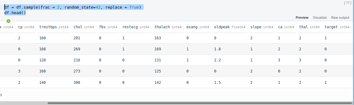
    df = df.sample(frac = 2, random_state=42, replace = True)
    df.head()

After this, when we analyse the dataset, we see random distribution of 0's and 1's in the target variable. Now, what we do is see if there are any null or missing value in the dataset.

    df.isnull().sum()

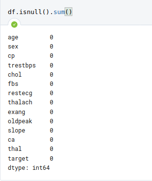Here, we can see that, there are no null values.

Now we are set to go for machine Learning Tasks

First we import required modules.

    #Import Machine Learning Libraries
    from sklearn.model_selection import train_test_split
    from sklearn import svm 
    from sklearn.model_selection import RandomizedSearchCV

The required modeules are imported. train_test_split is for dividing the dataset into training and testing sub-dataset. The svm is Support Vector Machine Algorithm. The RandomizedSearchCV is for hyperparameter Tuning. Alternative to RandomizedSearchCV is GridSearchCV, however RandomizedSearchCV is likely to be faster than GridSearchCV.

    X = df.drop(['target'], 1)
    y = df.target
    print(X.shape, y.shape)

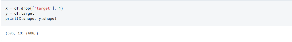Then we created a dataframe X which consists of Feature Variables, target is dropped because it is not Feature variable, rather it is target variable. y is defined as pandas series object with target as it only feature.

    X_train, X_test, y_train, y_test = train_test_split(X, y, test_size=0.2)
    clf = svm.SVC()
    clf.fit(X_train, y_train)
    print("The accuracy of the classifier is {}".format(clf.score(X_test, y_test)))

In this step, we divided X, y into train and test sub-dataset. train_test_split returns four objects, so we stored those values into X_train, X_test, y_train, y_test. The parameters are X, y, and the test_size=0.2 parameters defines what percentage of dataset is to be described for test_set which in this case are X_test and y_test. then we instantiated SVC (Support vector Classifier) into vairable clf and used fit() method to fit, X_train and y_train. The accuracy of the classifier is found to be mere 68.85%.

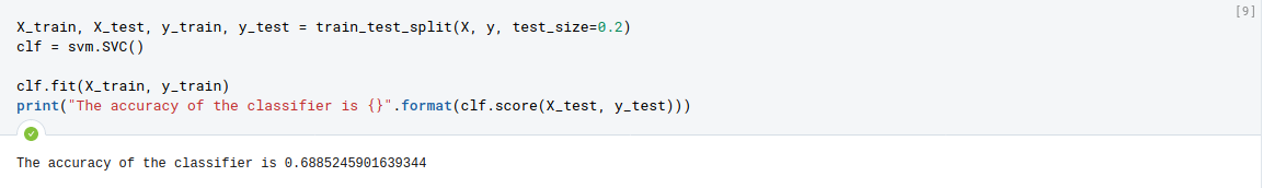Sadly, 68.85% percentage accuracy is very less, so we try to tune certain parameters and improve the accuracy.

#Lets try tuning some hyperparameters.
    param_dist = {'C': [0.1, 1, 10, 100, 1000],
    'gamma': [1, 0.1, 0.01, 0.001, 0.0001],
    'kernel': ['rbf']
    }
    svc_hyper = RandomizedSearchCV(SVC(), param_distributions=param_dist, verbose=2, cv=3, random_state=42, n_iter=10, scoring='accuracy')
    svc_hyper.fit(X_train, y_train)

Here, we used different set of parameters like C, gamma and kernel to loop through set of combinations of prameters and at the end define which set of combination of these parameters gives the best result. Here C is Regularization parameter. The strength of the regularization is inversely proportional to C. Must be strictly positive. The penalty is a squared l2 penalty. The parameter gamma is Kernel coefficient for ‘rbf’, ‘poly’ and ‘sigmoid’. And the parameter kernel Specifies the kernel type to be used in the algorithm. It must be one of ‘linear’, ‘poly’, ‘rbf’, ‘sigmoid’, ‘precomputed’ or a callable. If none is given, ‘rbf’ will be used. Here, we used only 'rbf' because other kernel takes significant time to get trained. You, yourself can try other kernels and see if that changes the results. To know more about SVC, go through this.

    svc_hyper.best_params_

we get the best parameter as {'kernel': 'rbf', 'gamma': 0.001, 'C': 1000}. So, lets use it to fit the data.

    best_svc = SVC(C=1000, gamma=0.001, kernel='rbf')
    best_svc.fit(X_train, y_train)
    print("The accuracy of the classifier is {}".format(best_svc.score(X_test, y_test)))

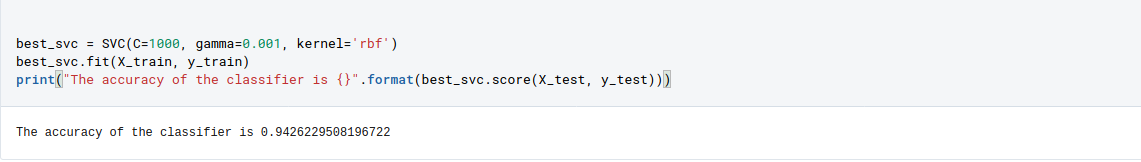After fitting the data using SVC method and using the best parameter, we got the accuracy to be 94.26%. That's remarkable to what we observe at first place as 68.85%.

Hence in this way, we can use RandomizedSearchCV to tune the parameters and increase the accuracy.

GitHub Repo of the code: github.com/bibekebib/Hyperpramater-tuning-a..

Deepnote Shared code: deepnote.com/@bibek-chalise/Hyperparameters..

If you want to try this with other Algoithms, here is a list of parameters that you can hypertune.

    #Random Forest 
    n_estimator = [int(x) for (x) in np.linspace(100, 1200, num=12)]
    max_depth = [int(x) for x in np.linspace(5, 30, num=6)]     
    min_samples_split = [2, 5, 10, 15, 100]
    min_samples_leaf = [1, 2, 5, 10] criterion = ['gini', 'entropy']
    param_dist = { "n_estimators" : n_estimator, "max_depth" : max_depth, "min_samples_leaf":min_samples_leaf, "criterion":criterion, "min_samples_split":min_samples_split }

    #KNN
    n_neighbors = [int(x) for x in np.linspace(start = 1, stop = 100, num = 50)]
    weights = ['uniform','distance'] 
    metric = ['euclidean','manhattan','chebyshev','seuclidean','minkowski'] 
    random_grid = { 'n_neighbors': n_neighbors, 'weights': weights, 'metric': metric, }

    #Logistic Regression
    param_dist = { 'penalty' : ['l1', 'l2'], 
    'C' : [0, 1, 2, 3, 4] 
    }

    #Gaussian Naive
    params_NB = {'var_smoothing': np.logspace(0,-9, num=100)}

Happy Learning!