Introduction

Hello everyone, welcome to my Blog in today's tutorial, we will be designing a more advanced ANN for image classification. So, this will be the subsequent part of our series on Computer Vision With PyTorch. So without a due, let's dive into the code.

So, this part of our code will be the same till download our dataset and create a data loader. If you are unclear about any step, I highly recommend you to check the tutorial, where I have explained all about it.

import torch
import torch.nn as nn
import torch.optim as optim
import torchvision
import torchvision.transforms as transforms
from torch.utils.data import DataLoader
import matplotlib.pyplot as plt

# Data preprocessing and augmentation
transform = transforms.Compose([
    transforms.ToTensor(),
    transforms.Normalize(mean=[0.5, 0.5, 0.5], std=[0.5, 0.5, 0.5])
])

# Load CIFAR-10 dataset
train_dataset = torchvision.datasets.CIFAR10(root='./data', train=True, download=True, transform=transform)
train_loader = DataLoader(train_dataset, batch_size=batch_size, shuffle=True)

Now, we need to define our model which will be structured in the same way as was previous tutorial but will have more layers.

class AdvancedANN(nn.Module):
    def __init__(self):
        super(AdvancedANN, self).__init__()
        self.fc1 = nn.Linear(32 * 32 * 3, 1024)
        self.fc2 = nn.Linear(1024, 512)
        self.fc3 = nn.Linear(512, 256)
        self.fc4 = nn.Linear(256, 128)
        self.fc5 = nn.Linear(128, 64)
        self.fc6 = nn.Linear(64, 10)
        self.relu = nn.ReLU()

    def forward(self, x):
        x = x.view(x.size(0), -1)  # Flatten the input images
        x = self.relu(self.fc1(x))
        x = self.relu(self.fc2(x))
        x = self.relu(self.fc3(x))
        x = self.relu(self.fc4(x))
        x = self.relu(self.fc5(x))
        x = self.fc6(x)
        return x

Here, our 3*32*32 image is converted to a 1-dimensional vector of 3072*1 and feed into the network. Then, it is projected to 1024 nodes followed by 512, 256, 128, 64 nodes and finally we have projected to 10 nodes because we have 10 classes in our dataset. The same is in the forward function, the view function is for reshaping the image into a single dimension, that's how we do reshaping in PyTorch.

# Hyperparameters
batch_size = 64
learning_rate = 0.001
num_epochs = 10

# Initialize the model
model = AdvancedANN()
# Define loss function and optimizer
criterion = nn.CrossEntropyLoss()
optimizer = optim.Adam(model.parameters(), lr=learning_rate)

This is also the same as the previous, just we will be using Adam as optimizer instead of SGD. Now, we need to define our training loop.

losses = []
accuracies = []
# Training loop
for epoch in range(num_epochs):
    model.train()  # Set the model to training mode
    total_correct = 0
    total_samples = 0
    total_loss = 0.0
    for i, (images, labels) in enumerate(train_loader):
        optimizer.zero_grad()
        outputs = model(images)
        loss = criterion(outputs, labels)
        loss.backward()
        optimizer.step()

        _, predicted = torch.max(outputs, 1)
        total_samples += labels.size(0)
        total_correct += (predicted == labels).sum().item()
        total_loss += loss.item()

        if (i + 1) % 100 == 0:
            print(f"Epoch [{epoch + 1}/{num_epochs}], Step [{i + 1}/{len(train_loader)}], Loss: {loss.item():.4f}")

    # Calculate and print accuracy
    accuracy = 100 * total_correct / total_samples
    print(f"Epoch [{epoch + 1}/{num_epochs}], Training Accuracy: {accuracy:.2f}%")

    # Calculate and store average loss and accuracy for the epoch
    average_loss = total_loss / len(train_loader)
    losses.append(average_loss)
    accuracies.append(accuracy)

print("Training finished.")

I have just added two new lists and appended the loss and accuracy of each epoch to plot them at the end of this training loop. so, if we run the cell, the training loop starts.

Epoch [1/10], Step [100/782], Loss: 1.7972
Epoch [1/10], Step [200/782], Loss: 1.6378
Epoch [1/10], Step [300/782], Loss: 1.8636
Epoch [1/10], Step [400/782], Loss: 1.7561
Epoch [1/10], Step [500/782], Loss: 1.5374
Epoch [1/10], Step [600/782], Loss: 1.3903
Epoch [1/10], Step [700/782], Loss: 1.9298
Epoch [1/10], Training Accuracy: 37.66%
Epoch [2/10], Step [100/782], Loss: 1.4052
Epoch [2/10], Step [200/782], Loss: 1.5323
Epoch [2/10], Step [300/782], Loss: 1.4231
Epoch [2/10], Step [400/782], Loss: 1.4050
Epoch [2/10], Step [500/782], Loss: 1.6354
Epoch [2/10], Step [600/782], Loss: 1.5001
Epoch [2/10], Step [700/782], Loss: 1.4958
Epoch [2/10], Training Accuracy: 47.43%
Epoch [3/10], Step [100/782], Loss: 1.4195
Epoch [3/10], Step [200/782], Loss: 1.4136
Epoch [3/10], Step [300/782], Loss: 1.3760
Epoch [3/10], Step [400/782], Loss: 1.3983
Epoch [3/10], Step [500/782], Loss: 1.4408
Epoch [3/10], Step [600/782], Loss: 1.5327
Epoch [3/10], Step [700/782], Loss: 1.4464
Epoch [3/10], Training Accuracy: 52.01%
Epoch [4/10], Step [100/782], Loss: 0.9776
Epoch [4/10], Step [200/782], Loss: 1.3968
Epoch [4/10], Step [300/782], Loss: 1.2217
Epoch [4/10], Step [400/782], Loss: 1.2327
Epoch [4/10], Step [500/782], Loss: 1.2769
Epoch [4/10], Step [600/782], Loss: 1.2474
Epoch [4/10], Step [700/782], Loss: 1.2011
Epoch [4/10], Training Accuracy: 55.39%
Epoch [5/10], Step [100/782], Loss: 1.4723
Epoch [5/10], Step [200/782], Loss: 1.3214
Epoch [5/10], Step [300/782], Loss: 1.2499
Epoch [5/10], Step [400/782], Loss: 1.0077
Epoch [5/10], Step [500/782], Loss: 1.2315
Epoch [5/10], Step [600/782], Loss: 1.3217
Epoch [5/10], Step [700/782], Loss: 0.9848
Epoch [5/10], Training Accuracy: 58.57%
Epoch [6/10], Step [100/782], Loss: 0.9484
Epoch [6/10], Step [200/782], Loss: 1.0160
Epoch [6/10], Step [300/782], Loss: 0.9097
Epoch [6/10], Step [400/782], Loss: 1.1121
Epoch [6/10], Step [500/782], Loss: 1.0643
Epoch [6/10], Step [600/782], Loss: 1.1222
Epoch [6/10], Step [700/782], Loss: 0.9151
Epoch [6/10], Training Accuracy: 61.42%
Epoch [7/10], Step [100/782], Loss: 1.0603
Epoch [7/10], Step [200/782], Loss: 0.9580
Epoch [7/10], Step [300/782], Loss: 1.1307
Epoch [7/10], Step [400/782], Loss: 0.9121
Epoch [7/10], Step [500/782], Loss: 0.8515
Epoch [7/10], Step [600/782], Loss: 0.8278
Epoch [7/10], Step [700/782], Loss: 0.9549
Epoch [7/10], Training Accuracy: 64.02%
Epoch [8/10], Step [100/782], Loss: 0.7921
Epoch [8/10], Step [200/782], Loss: 0.9545
Epoch [8/10], Step [300/782], Loss: 0.7991
Epoch [8/10], Step [400/782], Loss: 1.0606
Epoch [8/10], Step [500/782], Loss: 1.2592
Epoch [8/10], Step [600/782], Loss: 0.9369
Epoch [8/10], Step [700/782], Loss: 0.9270
Epoch [8/10], Training Accuracy: 67.04%
Epoch [9/10], Step [100/782], Loss: 0.7501
Epoch [9/10], Step [200/782], Loss: 1.1043
Epoch [9/10], Step [300/782], Loss: 0.8589
Epoch [9/10], Step [400/782], Loss: 1.1142
Epoch [9/10], Step [500/782], Loss: 0.7783
Epoch [9/10], Step [600/782], Loss: 0.9715
Epoch [9/10], Step [700/782], Loss: 0.8937
Epoch [9/10], Training Accuracy: 69.46%
Epoch [10/10], Step [100/782], Loss: 0.5709
Epoch [10/10], Step [200/782], Loss: 0.5713
Epoch [10/10], Step [300/782], Loss: 0.9997
Epoch [10/10], Step [400/782], Loss: 0.6164
Epoch [10/10], Step [500/782], Loss: 1.0069
Epoch [10/10], Step [600/782], Loss: 1.1473
Epoch [10/10], Step [700/782], Loss: 0.6924
Epoch [10/10], Training Accuracy: 71.88%
Training finished.

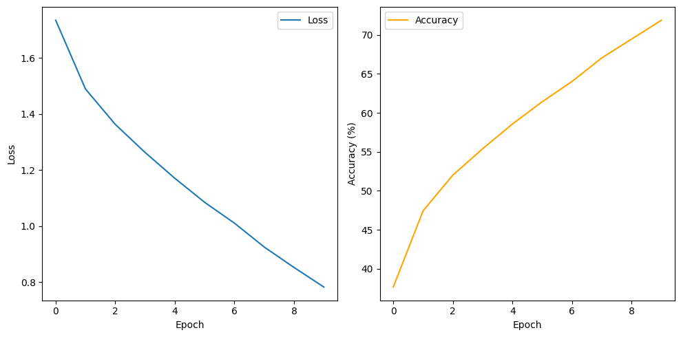
With the same dataset, however, with different architecture, we have been able to increase the accuracy and decrease loss.

# Save the trained model
torch.save(model.state_dict(), "advanced_ann_cifar10.pth")

In this step, we will be saving the trained model, and .pth is the extension for PyTorch model, .pt can also be used instead. We will talk about loading a saved model in upcoming tutorials and using it to predict non-trained data.

Now, let's plot a line plot for loss and accuracy.

# Plotting loss and accuracy
plt.figure(figsize=(10, 5))
plt.subplot(1, 2, 1)
plt.plot(losses, label='Loss')
plt.xlabel('Epoch')
plt.ylabel('Loss')
plt.legend()

plt.subplot(1, 2, 2)
plt.plot(accuracies, label='Accuracy', color='orange')
plt.xlabel('Epoch')
plt.ylabel('Accuracy (%)')
plt.legend()

plt.tight_layout()
plt.show()

conclusion

In this Tutorial, I have explained how to build an advanced artificial neural network from scratch with PyTorch. We learnt that with an increase in the number of layers, the overall performance of the model can be enhanced. But let me remind you just to get better results, we will not be increasing more and more layers. There are other ways to do that and we will talk about it in the upcoming days.