Introduction

Hello everyone, it's me Bibek Chalise and welcome to my Blog Series. In this tutorial, we will start a new series of tutorials and that will be Computer Vision with PyTorch. PyTorch is one of the machine learning frameworks and is based on Torch Library, and makes Computer Vision, Natural Language Processing and other machine learning and deep learning tasks easier. So, from today we will focus on using Computer Vision with PyTorch and I am assuming that you know a bit about computer vision background and PyTorch fundamentals like tensors and basic Neural Network stuff. But, if you don't know that too, we will slowly get to know about that stuff too. It's going to be a good series to cover up and finish. In this blog, we will be designing a very simple Artificial Neural Network to classify 10 different classes from very popular CIFAR-10 dataset. We will be downloading it from torchvision dataset hub, so there will be no fancy loading of our custom datasets in this particular video. But will do that for sure in upcoming videos. However, before starting the code, we need to understand a bit about how we are going to approach this task.

What is ANN?

Figure: Artificial Neural Network architectural diagram [source_image] ANNs (also called Artificial Neural Networks or simply neural networks), are computing systems vaguely inspired by the biological neural networks that learn from the data we feed them. So, in this case, since we will be feeding them images, they will learn patterns in the images and the classes associated with that pattern.

This tutorial is also available in Youtube in my youtube Channel.

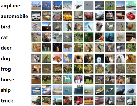
This is a sample of the dataset, so with each image of airplane we feed in the network, it generates a pattern for aeroplanes like it has two wings, metal like body and any other specific, we let the network decide what pattern to learn and whenever a new image is a feed into the network, it analyzes the pattern in the new test data and aligns with the pattern it previously learnt and gives us a probability result class.

What next?

So, I think we have a basic overview of what ANN is and how it will work. But how do we give our image of size 32*32 (Height and weight) coloured (3 channels) images to the Neural Network in such a way that it generalizes a pattern? In this case, what we need is to flatten this image to a single dimension. So, the 3 * 32 * 32 image of 3 dimensions will be converted to reshaped as 3072 * 1 dimensional vector. So we will have 3072 nodes as input nodes and will be projected to a definite number of nodes in the hidden layer.

Without further due, let's dive directly into the code. We will continue to know more about the structure along with the code in the video. Also, I am assuming you are well familiar with Google Colab, since we will be using that for this tutorial.

First of all, we need to import important libraries.

import torch
import torchvision
import torchvision.transforms as transforms
import torch.nn as nn
import torch.optim as optim
import torch.nn.functional as F

The torch is the main library of the PyTorch framework and torchvision is another PyTorch library for all computer vision tasks. Transforms will be used for any kind of data transformation or augmentation in the images, torch.nn will be the core Neural network class of Torch, torch.optim will be for Optimisers and torch.nn.functional has many functions that will be useful as we progress in the series.

# Define data transformations
transform = transforms.Compose([
    transforms.ToTensor(),
    transforms.Normalize((0.5, 0.5, 0.5), (0.5, 0.5, 0.5))  # Normalize images to [-1, 1]
])

In this cell, what we are trying to do is transforms the image to tensor, since PyTorch requires the values to be a Tensor, (like ndarray of Numpy), and ToTensor converts the image values in the range of 0 to 1. Then we normalize them with a mean 0.5 and 0.5 standard deviation for each channel, Remember we are working with RGB images, right?

# Load CIFAR-10 dataset
dataset = torchvision.datasets.CIFAR10(root='./cifar', train=True, transform=transform, download=True)
dataloader = torch.utils.data.DataLoader(dataset, batch_size=64, shuffle=True)

It's funny right, we have described how we will be going to transform our images but haven't loaded the images in our working directory. torchvision.datasets has many working datasets and we have chosen CIFER10 and we have downloaded it to ./cifer folder with parameter download=True. The train=True downloads only the train dataset from the hub whereas, transform=transform makes all the transformations to the downloaded images as described above. The Dataloader function helps us to feed inputs to the model in the batch of 64 images at one time.

class SimpleANN(nn.Module):
    def __init__(self):
        super(SimpleANN, self).__init__()
        self.fc1 = nn.Linear(3 * 32 * 32, 128)  # Flatten the 32x32 RGB images
        self.fc2 = nn.Linear(128, 64)
        self.fc3 = nn.Linear(64, 10)  # Output layer for 10 classes

    def forward(self, x):
        x = x.view(-1, 3 * 32 * 32)  # Flatten the input images
        x = F.relu(self.fc1(x))
        x = F.relu(self.fc2(x))
        x = self.fc3(x)
        return x

Now the big game time, we define our model. We make a Python class named SimpleANN and it is a subclass of nn.Module class which is the base class for all the Neural Network modules in PyTorch. The __init__(self) method called whenever SimpleANN class is called. So as I mentioned, we are converting the size of our image 3 * 32 * 32 into a one-dimensional vector and feeding as input to the ANN. Then, we connect that with 128 nodes in the first hidden layer, then that is connected to 64 nodes in the second hidden layer and finally we have 10 nodes as output layer for each of the 10 output classes.

The forward function is the forward pass to carry the input image through all the layers. In the forward layer, we have used Rectified Linear Unit or ReLU has been used which is a popular Activation Function which takes the input and outputs the input in between the maximum of 0 or input. So, this keeps non-linearity in the network to improve the performance of the network.

model = SimpleANN()
criterion = nn.CrossEntropyLoss()
optimizer = optim.SGD(model.parameters(), lr=0.001, momentum=0.9)

Now, we need to call the instance of SimpleANN class and we created a model as its instance. Also, we defined CrossEntropyLoss is our loss function which is used to calculate the loss during each training epoch and SGD or Stochastic Gradient Descent is used as our optimizer to update the weights of our network. So, lr=0.001 is the learning rate and defines the rate at which the weights are updated. The momentum parameter is to help us accelerate convergence.

# Training loop with accuracy calculation
epochs = 10
for epoch in range(epochs):
    running_loss = 0.0
    correct = 0
    total = 0
    for i, data in enumerate(dataloader, 0):
        inputs, labels = data
        optimizer.zero_grad()
        outputs = model(inputs)
        loss = criterion(outputs, labels)
        loss.backward()
        optimizer.step()
        running_loss += loss.item()

        # Calculate accuracy
        _, predicted = torch.max(outputs.data, 1)
        total += labels.size(0)
        correct += (predicted == labels).sum().item()

        if i % 100 == 99:
            print(f'Epoch {epoch + 1}, Mini-batch {i + 1}, Loss: {running_loss / 100:.3f}, Accuracy: {(100 * correct / total):.2f}%')
            running_loss = 0.0

print('Finished Training')

So, now we are in the training loop. we have chosen epochs=10 and in each epoch, we are taking 64 images and their corresponding labels from the data loader. Then, we feed that image to the model which gives us an output and we are only interested in the node which has the maximum probability. So, if the output is the same as the label, we increment it corret+1 and we calculate the accuracy. So, in this loop, there are a few things to understand.

    optimizer.zero_grad()
    outputs = model(inputs)
    loss = criterion(outputs, labels)
    loss.backward()
    optimizer.step()

So, here optimizer starts with zero gradients for each epoch and only after the calculation of loss by the difference between predicted output and labels, the backward propagation starts and the optimizer updates the weights as per the loss. We zero out all of our gradients so that they don't accumulate over time and then calculate new ones using a backpropagation algorithm.

Epoch 1, Mini-batch 100, Loss: 1.306, Accuracy: 54.05%
Epoch 1, Mini-batch 200, Loss: 1.324, Accuracy: 53.85%
Epoch 1, Mini-batch 300, Loss: 1.337, Accuracy: 53.52%
Epoch 1, Mini-batch 400, Loss: 1.318, Accuracy: 53.50%
Epoch 1, Mini-batch 500, Loss: 1.312, Accuracy: 53.63%
Epoch 1, Mini-batch 600, Loss: 1.308, Accuracy: 53.85%
Epoch 1, Mini-batch 700, Loss: 1.311, Accuracy: 53.88%
Epoch 2, Mini-batch 100, Loss: 1.315, Accuracy: 54.02%
Epoch 2, Mini-batch 200, Loss: 1.276, Accuracy: 54.66%
Epoch 2, Mini-batch 300, Loss: 1.287, Accuracy: 54.74%
Epoch 2, Mini-batch 400, Loss: 1.276, Accuracy: 54.80%
Epoch 2, Mini-batch 500, Loss: 1.311, Accuracy: 54.75%
Epoch 2, Mini-batch 600, Loss: 1.268, Accuracy: 54.96%
Epoch 2, Mini-batch 700, Loss: 1.275, Accuracy: 55.04%
Epoch 3, Mini-batch 100, Loss: 1.279, Accuracy: 55.28%
Epoch 3, Mini-batch 200, Loss: 1.265, Accuracy: 55.54%
Epoch 3, Mini-batch 300, Loss: 1.270, Accuracy: 55.62%
Epoch 3, Mini-batch 400, Loss: 1.259, Accuracy: 55.79%
Epoch 3, Mini-batch 500, Loss: 1.263, Accuracy: 55.89%
Epoch 3, Mini-batch 600, Loss: 1.248, Accuracy: 56.00%
Epoch 3, Mini-batch 700, Loss: 1.259, Accuracy: 55.91%
Epoch 4, Mini-batch 100, Loss: 1.223, Accuracy: 56.84%
Epoch 4, Mini-batch 200, Loss: 1.223, Accuracy: 57.07%
Epoch 4, Mini-batch 300, Loss: 1.229, Accuracy: 57.10%
Epoch 4, Mini-batch 400, Loss: 1.253, Accuracy: 56.86%
Epoch 4, Mini-batch 500, Loss: 1.218, Accuracy: 57.06%
Epoch 4, Mini-batch 600, Loss: 1.235, Accuracy: 56.99%
Epoch 4, Mini-batch 700, Loss: 1.252, Accuracy: 56.89%
Epoch 5, Mini-batch 100, Loss: 1.177, Accuracy: 58.47%
Epoch 5, Mini-batch 200, Loss: 1.215, Accuracy: 57.97%
Epoch 5, Mini-batch 300, Loss: 1.214, Accuracy: 58.03%
Epoch 5, Mini-batch 400, Loss: 1.162, Accuracy: 58.38%
Epoch 5, Mini-batch 500, Loss: 1.206, Accuracy: 58.28%
Epoch 5, Mini-batch 600, Loss: 1.215, Accuracy: 58.09%
Epoch 5, Mini-batch 700, Loss: 1.239, Accuracy: 57.92%
Epoch 6, Mini-batch 100, Loss: 1.188, Accuracy: 58.33%
Epoch 6, Mini-batch 200, Loss: 1.169, Accuracy: 58.79%
Epoch 6, Mini-batch 300, Loss: 1.165, Accuracy: 58.77%
Epoch 6, Mini-batch 400, Loss: 1.195, Accuracy: 58.73%
Epoch 6, Mini-batch 500, Loss: 1.184, Accuracy: 58.74%
Epoch 6, Mini-batch 600, Loss: 1.195, Accuracy: 58.55%
Epoch 6, Mini-batch 700, Loss: 1.199, Accuracy: 58.46%
Epoch 7, Mini-batch 100, Loss: 1.172, Accuracy: 59.00%
Epoch 7, Mini-batch 200, Loss: 1.157, Accuracy: 58.99%
Epoch 7, Mini-batch 300, Loss: 1.159, Accuracy: 59.08%
Epoch 7, Mini-batch 400, Loss: 1.158, Accuracy: 59.22%
Epoch 7, Mini-batch 500, Loss: 1.170, Accuracy: 59.25%
Epoch 7, Mini-batch 600, Loss: 1.174, Accuracy: 59.15%
Epoch 7, Mini-batch 700, Loss: 1.159, Accuracy: 59.12%
Epoch 8, Mini-batch 100, Loss: 1.128, Accuracy: 60.77%
Epoch 8, Mini-batch 200, Loss: 1.124, Accuracy: 61.12%
Epoch 8, Mini-batch 300, Loss: 1.133, Accuracy: 60.99%
Epoch 8, Mini-batch 400, Loss: 1.152, Accuracy: 60.70%
Epoch 8, Mini-batch 500, Loss: 1.140, Accuracy: 60.70%
Epoch 8, Mini-batch 600, Loss: 1.156, Accuracy: 60.41%
Epoch 8, Mini-batch 700, Loss: 1.172, Accuracy: 60.16%
Epoch 9, Mini-batch 100, Loss: 1.119, Accuracy: 61.19%
Epoch 9, Mini-batch 200, Loss: 1.120, Accuracy: 60.77%
Epoch 9, Mini-batch 300, Loss: 1.132, Accuracy: 60.68%
Epoch 9, Mini-batch 400, Loss: 1.106, Accuracy: 60.84%
Epoch 9, Mini-batch 500, Loss: 1.125, Accuracy: 60.79%
Epoch 9, Mini-batch 600, Loss: 1.139, Accuracy: 60.73%
Epoch 9, Mini-batch 700, Loss: 1.118, Accuracy: 60.79%
Epoch 10, Mini-batch 100, Loss: 1.088, Accuracy: 61.70%
Epoch 10, Mini-batch 200, Loss: 1.074, Accuracy: 61.97%
Epoch 10, Mini-batch 300, Loss: 1.103, Accuracy: 61.71%
Epoch 10, Mini-batch 400, Loss: 1.090, Accuracy: 61.99%
Epoch 10, Mini-batch 500, Loss: 1.121, Accuracy: 61.59%
Epoch 10, Mini-batch 600, Loss: 1.113, Accuracy: 61.45%
Epoch 10, Mini-batch 700, Loss: 1.100, Accuracy: 61.44%
Finished Training

This is the result of the training loop and at the end of 10 epochs, we achieved a loss of 1.1 and loss of 61.44%. This was the simplest Neural Network designed, so we can tweak over optimizer type, number of epochs, batch_size, and number of layers in the architecture of the ANN. In the next tutorial, we will be looking at the design of a more complex ANN for a new dataset and see how a change in architecture makes an impact on the overall performance of the model. So, until, then I sign off from this tutorial and see you again.

References

• PyTorch Tutorials

• source_image

• ColabNotebook