Introduction

Hello everyone, welcome to my Blog in this tutorial, we will be learning how to do simple image classification as we did in the last tutorial but this time, we will be leveraging PyTorch Lightning to do the same task but with ease. So, I am planning to release both core PyTorch implementation as well as PyTorch Lightning implementation.

Without much due, let's dive directly into the code.

In Local Machine

    pip3 install lightning

In Colab Notebook

    !pip install lightning

At first, we need to install lightning in our device. For this tutorial, we will be using Colab, and in colab also we have to install it.

import os
import torch
from torch import nn
import torchvision
import torch.nn.functional as F
from torchvision import transforms
from torch.utils.data import DataLoader
import lightning.pytorch as pl

So, all the required modules are imported. Everything looks almost the same, just the import of lightning.pytorch as pl is new. Then, let's copy a few more lines from previous tutorials, nothing new, the same lines and the same function.

# Data preprocessing and augmentation
transform = transforms.Compose([
    transforms.ToTensor(),
    transforms.Normalize(mean=[0.5, 0.5, 0.5], std=[0.5, 0.5, 0.5])
])

# Load CIFAR-10 dataset
dataset = torchvision.datasets.CIFAR10(root='./cifar', train=True, transform=transform, download=True)
dataloader = torch.utils.data.DataLoader(dataset, batch_size=64, shuffle=True)

criterion = nn.CrossEntropyLoss()

The model definition will also be the same.

class SimpleANN(nn.Module):
    def __init__(self):
        super(SimpleANN, self).__init__()
        self.fc1 = nn.Linear(3 * 32 * 32, 128)  # Flatten the 32x32 RGB images
        self.fc2 = nn.Linear(128, 64)
        self.fc3 = nn.Linear(64, 10)  # Output layer for 10 classes

    def forward(self, x):
        x = x.view(-1, 3 * 32 * 32)  # Flatten the input images
        x = F.relu(self.fc1(x))
        x = F.relu(self.fc2(x))
        x = self.fc3(x)
        return x

class LitSimpleANN(pl.LightningModule):
  def __init__(self, model):
    super().__init__()
    self.model = model

  def training_step(self, batch, batch_idx):
    x, y = batch
    # print(y)
    out = self.model(x)
    # print(out)
    loss = criterion(out, y)
    preds = torch.argmax(out, dim=1)
    accuracy = torch.sum(preds == y).item() / y.size(0)

    self.log('train_loss', loss,  on_epoch=True)  # Log training loss
    self.log('train_accuracy', accuracy,  on_epoch=True)
    return loss

  def configure_optimizers(self):
    optimizer = torch.optim.SGD(self.model.parameters(), lr=0.001, momentum=0.9)
    return optimizer

Now, the real magical lines of PyTorch lightning come into action. We defined a class LitSimpleANN as a subclass of PyTorch Lightning Module and this class takes the above-defined SimpleANN class as input. Then, we define the training step inside this LitSimpleANN class. training_step function takes batch and batch_idx as input. So each batch has input images and the labels associated with the batch. So, Same as before, we fed the model the input image, it gives the probability distribution of each class and we calculate loss and accuracy on it. Here, self.log stores loss and accuracy per step and per epoch which can be useful during the evaluation of the model performance.

model = LitSimpleANN(SimpleANN())

Training the data

from pytorch_lightning.loggers.csv_logs import CSVLogger

trainer = pl.Trainer(max_epochs=10,  logger=CSVLogger("logs"))
trainer.fit(model = model, train_dataloaders=dataloader)

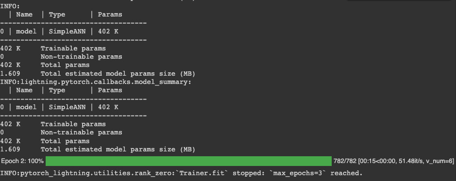
Here, I have imported CSVLogger to save the logs in CSV format for further reference. Here, pl.Trainer takes away all the manual training loops from the custom PyTorch training loop we also discussed in the last video. So, when we hit shift enter, Bam, the training starts. Nothing much fancy here, max_epochs=10 is for the number of epochs, as the default is 1000 epochs. The output of this code is as follows:

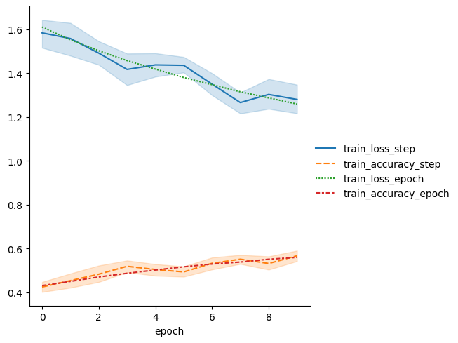
Let's plot some graphs.

import pandas as pd
import seaborn as sn
metrics = pd.read_csv(f"{trainer.logger.log_dir}/metrics.csv")
del metrics["step"]
metrics.set_index("epoch", inplace=True)
sn.relplot(data=metrics, kind="line")

The mertics.csv is auto-generated by trainer logger and this will give a nice line graph.

Conclusion

In this post, we learned how to implement image classification using simple ANN in the PyTorch Lightning library. Lightening AI is fast, easy to use and saves us from unnecessary loops of code. I highly recommend you all learn about it and it will save you from hassle compared to core PyTorch code.

This much from today, so see you guys in the next tutorial.

Colab

YouTube

Bibek Chalise is a Machine Learning enthusiast, Computer Vision Scientist and is associated with MarginTop Solutions.

MarginTop Solutions

Where Tech Meets Brilliance

Pokhara, Nepal

margintopsolutions@gmail.com

Website